Math of Freeciv/Battle outcome

This page describes in mathematical terms what will be the result of one unit attacking another.

Probability of winning a fight

The chances of winning a fight are sometimes counter-intuitive. E.g., what would you say are your chances of winning in the following situation (after taking into account the land advantages and other modifiers): you have an attack of 2 against a defense of 3, and the same number of hit points? Considering that the probability of winning each round is 2/5, you might think that this will give you with a reasonable chance of victory, something like 40%. Lost. You only have 19% chances of winning. The fact that the battle lasts several rounds tends to give a larger advantage to the biggest power than one could think beforehand.

Supposing the reader is aware of the rules of the fight (for each round, take a random number, decide who wins that round, etc.), let's try to find a formula representing the chances of victory.

Notations and basic computations

Consider a unit having a strength (all modifications, field, city, unit experience of combat, etc. being applied) $s$ and an enemy unit having a defense $r$. The number of hit points of the defending unit is written $d_\text{hp}$ , the damages per victorious rounds from the attacking unit is $a_\text{fp}$ .

Let us note $k$ the number of victorious rounds required to win the fight. And $l$ is the number of rounds that, if lost, implies a defeat ($l$ is for "losing allowance"). When the attacking unit cause one damage per victorious rounds ($a_\text{fp}=1$), $k$ is the number of hit points of the defending unit ($d_\text{hp}$). More generally,

$k=\left\lfloor {\frac {d_{\text{hp}}+a_{\text{fp}}-1}{a_{\text{fp}}}}\right\rfloor =\left\lceil {\frac {d_{\text{hp}}}{a_{\text{fp}}}}\right\rceil$.

$l$ may be computed similarily. The chance of winning each round, let us note it $p$ , is

$p = \frac{s}{s+r}$.

Thus the chance of losing a round is

$q=1-p$.

Let us also denote $m$ the maximal possible number of rounds fought. Usually, since each round results in some unit's loss of points and after a unit is defeated it can't strike any more and its enemy must keep at least one point, and the total number of possible losses is $k+l$, $m$ is equal to

$m_{d}=k+l-1$

(variant of when it happens: attacker loses $l-1$ round and then wins until the victory). But since version 3.0 of Freeciv this number can be limited by ruleset; so, if $m<k+l-1$, there is some probability that both units survive the battle (limitation greater than or equal to $m_d$ has no effect).

Reasoning

Now let us suppose that the fight takes $n$ rounds to achieve, and let us compute the probability of victory. Note that we do not know $n$ in advance but we suppose for now that it is given. For a given $n$, the probability of victory is the probability that $k$ rounds have been won over these $n$ tries and less than $l$ rounds have been lost. If $n < k + l$, then the probability of victory is simply the probability that $k$ rounds have been won over these $n$ tries (as this implies that less than $l$ rounds have been lost). In case of victory, the last round must be the final hit (otherwise the fight would have been stopped earlier). Apart from that, there must be $k - 1$ hits among the $n-1$ other rounds. That probability is given by a binomial $B(n-1,p)$ and is

${n-1 \choose k-1}p^{k-1}q^{n-k}$.

As the last round must be won, we multiply by $p$ and get a probability of victory with $n$ rounds of

$P_{Wn}={n-1 \choose k-1}p^{k}q^{n-k}$.

For the attacking unit to win the fight, we must have (assuming that $m=m_{d}$)

$k \leq n < k + l$.

Thus finally the probability of winning equals:

$P_{W}=\sum _{n=k}^{k+l-1}{n-1 \choose k-1}p^{k}q^{n-k}$.(1)

Reasoning from the defeat count

The freeciv source code uses a slightly different reasoning (look at ./common/combat.c:unit_win_chance() and ./common/combat.c:win_chance()). Let us note $d$ the number of rounds lost, which must be smaller than $l$ for a victorious attack. Then we have the following probability of victory:

$P_{W}=\sum _{d=0}^{l-1}{k-1+d \choose d}p^{k-1}q^{d}p$.(2)

We get the formula (1) by using

$n = k + d$

and

${n-1 \choose n-k} = {n-1 \choose k-1}$.

In the code,

$k$ is def_N_lose,

$l$ is att_N_lose,

$p$ is def_P_lose1,

$(1-p)$ is att_P_lose1,

$d$ is lr.

Round limit is not currently taken into account in the code, but probably some day it will be.

Generalized reasoning

Let's imagine that the fight always consists of $m$ rounds, even if usually one of the parts in reality is killed before the number is reached; we now have a set of $2^m$ different imaginary battles. All the real fights have one or more items in this set for which actual rounds are matching real ones and the remaining ones are any possible sequence (for $n$-round battle, there are $2^{m-n}$ matching items). We can see that probability of the imaginary subset is equal to the probability of the real battle it matches (since first rounds are similar, following imaginary rounds are independent, and happening of any one of all possible combinations has the possibility of $1$). Then, any sequence where $k$ or more rounds are win matches to a won fight, and any one that has $l$ or more rounds lost matches a lost fight (because $m\leq m_{d}<k+l$, imaginary fight can't have $l$ losses when in its real part there are $k$ wins, etc.) Thus, we come again to the Bernoulli model: the probability of victory is equal to the probability of having $k$ or more successes in $B(m,p)$ series. This can be expressed using Bernoulli cumulative distribution function (possibility of getting $k$ or less successes)

$F_{B\;N,p}(k)=\sum _{i=0}^{k}{N \choose i}p^{i}(1-p)^{N-i}$:

the possibilities of winning, losing and "stalemate" are respectedly (if $l\leq m\geq k$)

$P_{W}=1-F_{B\;m,p}(k-1)=F_{B\;m,q}(m-k)$,

$P_{L}=1-F_{B\;m,q}(l-1)=F_{B\;m,p}(m-l)$,

Failed to parse (syntax error): {\displaystyle P_S=1-P_W-P_L=F_{B\;m,p}(k-1)-F_{B\;m,p}(m-l)=F_{B\;m,q}(l-1)-F_{B\;m,q}(m-k)\text.}

The equivalence of (1), (2) and this form (with $m=m_{d}$) which expands as

$P_{W}=1-\sum _{i=0}^{k-1}{m \choose i}p^{i}q^{m-i}=\sum _{i=k}^{m}{m \choose i}p^{i}q^{m-i}$,(3)

can be clearly shown by algebraic transformations, just nobody have done it here yet.

Approximate estimation of the winning chance

Binomial distributions are mathematicians' lab mice and are well studied, thus, fast approximate ways to estimate such chances are known. Binomial random values are subject to the central limit theorem, and $B(N,p)$ with sufficiently big $N$ approaches normal distribution $N(\mu =Np,\sigma ={\sqrt {npq}})$ (first parameter is the mean and the second is the standard deviation of both distributions). The normal distribution is scalable from the standard one $N(1,1)$ with cumulative function

$\Phi (x)=\int _{-\infty }^{x}{e^{-{x^{2} \over 2}} \over {\sqrt {2\pi }}}dx$,

so that with the scaling function $x(\alpha )={\frac {\alpha -\mu }{\sigma }}$

$F_{B\;N,p}(k)\approx \Phi (x(k-0.5))-\Phi (x(-0.5))$,

and thus

$P_{W}\approx 1-\Phi \left({k-mp-0.5 \over {\sqrt {mpq}}}\right)+\Phi \left({-mp-0,5 \over {\sqrt {mpq}}}\right)$.

Since $\Phi (x<-3)<0.0015$ and $\Phi (x>3)>0.9985$, we can be almost sure in the battle result if $\left|mp-k\right| \over {\sqrt {mpq}}$ is greater than 3 without extra computations. In the interval, the function $\Phi(x)$ is smooth and can be easily approximated by something fast.

The trouble is that if $p$ differs much from $0,5$, the $N$ big enough for any credible value of this approximation goes very big. Top estimation of the error is

$\Delta _{Nmax}=0.7655{\frac {p^{2}+q^{2}}{\sqrt {mpq}}}{\overset {p\ll 0,5}{\approx }}{\frac {0.7655}{\sqrt {mp}}}$.

Luckily, for small $p$'s works the Poisson distribution approximation $P(\lambda =Np)$, which parameter equals both mean and dispersion; for big possibilities, just switch $p$ with $q$. The function is

$F_{P\;\lambda }(k)=\sum _{i=0}^{k}{\frac {\lambda ^{k}e^{-\lambda }}{k!}}$,

$P_{W}{\overset {p\ll 0,5}{\approx }}1-F_{P\;mp}(k)$.

The error is limited by $\Delta _{Pmax}=\min(mp^{2},p)$. The Poisson distribution can't be scaled from a single curve, but the row itself is stabilizing fast enough. We can suggest which approximation is better by studying $\Delta _{Nmax}/\Delta _{Pmax}$. It's likely for $m > 1$ that when it is over 2.3 normal one is better, and when under 1.125, the Poisson one, and in the uncertain gap taking the average of both gives good estimation (especially if the possibility is smaller than 50% since in this region these approximations tend to errate in opposite directions), but this idea requires better mathematical founding. The precision considering this all is about ±4% absolute, and might fit ±0.5% interval for $m>10$.

Equivalent killer

Any attacker is characterized with three parameters - health $a_{\text{hp}}$, strength $s$ and firepower $a_{\text{hp}}$ (similar ones have each defender; here let's think that $m=k+l-1$). Two attackers with at least one different parameter won't attack targets in similar manner (prove yourself that the intuitive presumption "twice more fp with twice less strength gives likely similar damage" is false). We can consider an attack on a specific defender: what health should have an attacker of standard strength and firepower to kill it with the same probability as our one. For this purpose, consider a simplified normal approximation (reasonably precise for big $mq$): $P_{W}=1-P_{L}=F_{B\;m,q}(l-1)\approx \Phi \left({l-mq-1 \over {\sqrt {mpq}}}\right)$. The argument of the $\Phi$, say $x$, should be the same. Thus, we get new $l$ from the equation where we calculate $x$ for a real attacker and take $d_\text{hp}$ of an actual defender, and take another parameters for our standard attacker

${l-(k+l-1)q-1 \over {\sqrt {(k+l-1)pq}}}=x$

${\frac {\left((l-1)p-kq\right)^{2}}{(k+l-1)pq}}=x^{2}{\text{, remember that }}\mathrm {sign} ((l-1)p-kq)=\mathrm {sign} (x)$

$\left(l-1-{\frac {kq}{p}}\right)^{2}=x^{2}\left({\frac {kq}{p}}+(l-1){\frac {q}{p}}\right)$

$(l-1)^{2}-2\left({\frac {kq}{p}}+{\frac {x^{2}}{2}}\cdot {\frac {q}{p}}\right)(l-1)+\left({\frac {kq}{p}}\right)^{2}-{\frac {kq}{p}}x^{2}=0$

$l-1={\frac {kq}{p}}+{\frac {x^{2}}{2}}\cdot {\frac {q}{p}}\pm {\sqrt {\left({\frac {kq}{p}}-{\frac {x^{2}}{2}}\cdot {\frac {q}{p}}\right)^{2}-\left({\frac {kq}{p}}\right)^{2}+{\frac {kq}{p}}x^{2}}}=$

$={\frac {kq}{p}}+{\frac {x^{2}}{2}}\cdot {\frac {q}{p}}\pm {\sqrt {{\frac {x^{4}}{4}}\left({\frac {q}{p}}\right)^{2}+{\frac {kq}{p}}x^{2}{\frac {q}{p}}+{\cancel {\left({\frac {kq}{p}}\right)^{2}}}-{\cancel {\left({\frac {kq}{p}}\right)^{2}}}+{\frac {kq}{p}}x^{2}}}=$

$={\frac {kq}{p}}+x{\frac {q}{p}}\left({\frac {x}{2}}\pm {\sqrt {\left({\frac {x}{2}}\right)^{2}+{\frac {kq}{p}}\left(\left({\frac {q}{p}}\right)^{-1}+\left({\frac {q}{p}}\right)^{-2}\right)}}\right)$

We can clearly see (just move ${\tfrac {kq}{p}}$ to the left and understand that the bracketed expression is either always positive or always negative) that the "−" solution is false, so

$l=1+{\frac {q}{p}}k+x\left({\frac {q}{p}}\cdot {\frac {x}{2}}+{\sqrt {\left({\frac {q}{p}}\cdot {\frac {x}{2}}\right)^{2}+k\left(\left(q/p\right)^{2}+1\right)}}\right)$,

or, substituting the properties of the standard unit,

$l_{s,a_{\text{fp}}}(x)=1+{\frac {r}{s}}\left\lceil {\frac {d_{\text{hp}}}{a_{\text{fp}}}}\right\rceil +x\left({\frac {xr}{2s}}+{\sqrt {{\Big (}{\frac {xr}{2s}}{\Big )}^{2}+\left\lceil {\frac {d_{\text{hp}}}{a_{\text{fp}}}}\right\rceil \left(\left({\frac {r}{s}}\right)^{2}+1\right)}}\right)$.

This value probably needs rounding to integer and some iterative amendment due to approximation errors, but goes as a quick estimation. For example, to say approximately how many Warriors ($a_{\text{fp}}=1,s=1,a_{\text{hp}}=1$) are equal to one half-hitpoints Artillery ($a_{\text{fp}}=2,s=10,a_{\text{hp}}=10$) in attack on an elite Partisan ($d_{\text{fp}}=1,r=8,d_{\text{hp}}=20$), we calculate

$k=\lceil 20/2\rceil =10,\quad l=\lceil 10/1\rceil =10,\quad r/s=8/10=0.8$

$x={\frac {10-1-10\cdot 0.8}{\sqrt {(10-1+10)\cdot 0.8}}}=0.256,$

$l_{1,1}=1+8\cdot 20+0,256\cdot \left({\frac {0.256\cdot 8}{2}}+{\sqrt {\left({\frac {0.256\cdot 8}{2}}\right)^{2}+20\cdot (8^{2}+1)}}\right)=170.51\approx 171{\text{.}}$

Precise $P_{W}$ values (calculated with OOoCalc/Excel function BINOM.DIST, with $q=8/(8+10)=0.444$ for Artillery and $8/(8+1)=0.889$ for Warriors) are 0.689 and 0.635. Really, the best estimated "warrior worth" for Artillery here is 177 ($P_{W}=0.690$).

We can use the same formula for getting number and/or health (obviously, healthes of attackers with similar fp and strength are additive with rounding up to $d_{\text{fp}}$, i.e. $k$'s are additive) of any specific units which, being sent to conquer a specific target, do it with given probability; for that, we'll use inverted normal distribution function (NORM.S.INV) to get $x=\Phi ^{-1}(P_{W})$:

Failed to parse (syntax error): {\displaystyle n=\left\lceil l_{s,a_\text{fp}}|_{\Phi^{-1}(P_W)} \over \left\lceil a_\text{hp}/d_\text{fp}\right\rceil\right\rceil,\quad a_\text{hp}=d_\text{fp}\cdot l_{s,a_\text{fp}}|_{\Phi^{-1}(P_W)}} .

In the example above, using this function would give us $x=0.492$, $l_{1,1}=179.7\approx 180$ and $P_{W}|_{l_{1,1}}=0.715$ which is slightly more precise but slower to compute. Equivalently kiling attacker can be defined in this way also for units with limited round nuber, but results of their action are so different that it will have less sense.

Note the two things:

1. We need defender health (and other parameters) to convert attacker health.
2. We deliberately used an elite unit in the examle above to avoid dealing with veteran status.

Approximation using ratings

AI code likes to compare unit strengthes by their (unspecifoc, advisor's) attack/defense ratings $a_{r}=a_{\text{hp}}\cdot s\cdot a_{\text{fp}}{\text{, }}d_{r}=d_{\text{hp}}\cdot r\cdot d_{\text{fp}}$. Sometimes the code suggests that $P_{W}\approx {\frac {a_{r}^{2}}{a_{r}^{2}+d_{r}^{2}}}$ and that squared ratings of units acting together (without killstack rule involved) are additive. That is not perfectly precise in general but makes some sense.

Using a robust normal approximation, we get that

$P_{W}\approx \Phi \left({\frac {lp-kq}{\sqrt {(k+l)pq}}}\right)=\Phi \left({\frac {a_{r}-d_{r}}{\sqrt {a_{\text{fp}}d_{\text{fp}}(a_{r}r+d_{r}s)}}}\right)\approx \Phi \left({\frac {a_{r}/d_{r}-1}{\sqrt {a_{r}/d_{r}(1/k+1/l)}}}\right)$.

This function happens to look pretty much alike ${\frac {(a_{r}/d_{r})^{2}}{(a_{r}/d_{r})^{2}+1}}$ when $1/k+1/l\approx 0.79$ but only qualitive alike if this value significantly differs.

Sum of squared ratings has just that sense that it weights stronger units more than just a linear rating sum, so you see not only that one stack is going to beat the another but that many of its units may survive the battle that is usually the actually desired result. Really, if the deviation is relatively small, in a battle of 1 unit against n with the same summary rating usually one unit from either side survives, but for the side of one unit it's 100% and for the other side it's only 1 out of n, so for such battles you have to produce about $n^2$ times more smaller units to keep in line.

The remaining HP

Well, maybe you will win. But won't your victory be Pyrrhic? Will your Mech._Inf. after vanquishing Musketeers have enough HP remaining to defend the next turn from a pair of Warriors lurking nearby?

Unlimited match variant

Results of the experiment, 10 vs 10.
Artillery hp are 5, 4, 4, 7, 3, 3 (lost ave. 5.67hp, expected 5.97), Partisans' are 8, 4, 6, 10 (lost ave. 13.0, expected 13.75)

Using aforementioned symbols, we can express winning attacker's health points remaining from initial $a_{\text{hp}}$ after losing $d$ rounds to a defender with firepower $d_{\text{fp}}$

$a_{\text{hp}}'=a_{\text{hp}}-d\cdot d_{\text{fp}}$,

here $d\in [0;l-1]$. Probability of having at least $x,x\leq a_{\text{hp}}$ hp remained in case of a victory we can express modifying the (2) equation

Failed to parse (syntax error): {\displaystyle \mathrm P(a_\text{hp}'\ge x|\text{win}) = \mathrm P\left(d\le \left\lfloor \frac{a_\text{hp}-x}{d_\text{fp}}\right\rfloor=d_x\text{, suppose }d_x\le m|\text{win}\right)=\\ =\frac{1}{P_W}\sum_{d=0}^{d_x}{k - 1 + d \choose k-1} p^k q^d\text{.}}

The sum looks like the negative binomial distribution $\mathrm {NB} (k,p)$, that governs the number $d$ of failures in a binomial series before $k$ successes, which happen with probability $p$ on each test, are achieved:

$\mathrm {P} (a_{\text{hp}}'\geq x|{\text{win}})={\frac {1}{P_{W}}}F_{NB\;k,p}\left(\left\lfloor {\frac {a_{\text{hp}}-x}{d_{\text{fp}}}}\right\rfloor \right)$,

and the probability of losing specific number of rounds $d,0\leq d<l$

$\mathrm {P} (d)=f_{NB\;k,p}(d)={k-1+d \choose d}p^{k}q^{d}$.

Negative binomial distribution has mean ${\frac {kq}{p}}=k{\frac {r}{s}}$;. If $p \approx 1$ and the mean is moderate, then it can be approximated by Poisson distribution with the same parameter; if $p\approx 0.5$, it is closer to normal distribution with a varianse similar to its, which is $\sigma ^{2}={\frac {kq}{p^{2}}}$ (and for $k = 1$ the distribution becomes geometric regression). But it is defined to the infinity and what we have here has a truncation of results at $l$. The average number of lost round in case of a won battle, due to the properties of the truncated distribution, will be

$\langle d|d<l\rangle =k{\frac {q}{p}}-{\frac {{\frac {kl}{p}}f_{NB\;k,p}(l)}{kP_{W}}}={\frac {kq}{p}}-{\frac {lf_{NB\;k,p}(l)}{pP_{W}}}$

where the untruncated probability function at specific value

$f_{NB\;k,p}(d)={k-1+d \choose d}p^{k}q^{d}$.

Analogically, if the attacker loses, average damage that the defender suffers is

$\langle w|w<k\rangle ={\frac {lp}{q}}-{\frac {kf_{NB\;l,q}(k)}{qP_{L}}}$.

Note that equivalent killers are in general not equivalent damagers. In the example above, if Artillery loses, it reduces Partisan's hp (don't forget to multiply on $a_\text{fp}$) at average on 13.75, while hordes of 171, 177 and 180 Warriors do it respectively on 16.4, 16.56 and 16.64, leaving thus like a half less.

If we use the imaginary battle concept, winning after losing $d\leq d_{x}$ rounds is equivalent to winning $k$ or more rounds in a $k+d_{x}$-round battle, thus we can also express the cumulative damage distribution via positive binomial function with a sliding parameter

$\mathrm {P} (a_{\text{hp}}'\geq x|{\text{win}})={\frac {1}{P_{W}}}\sum _{i=k}^{k+d_{x}}{k+d_{x} \choose i}p^{i}q^{k+d_{x}-i}={\frac {1}{P_{W}}}\left(1-F_{B\;k+d_{x},p}(k-1)\right)$.

Limited match variant

Limited (15 rounds) match variant, same stats: Artillery (7*, 5*, 2, 6*, 2, 1, 5*, 8*, 8*, avg. 4.89, exp. 3.78), Partisans (6, 6, 8, 10*, avg. 7.50, exp. 5.22, some got a glitch in hitbar). * - killed the enemy (expected 7.1% Partisans and 27.5% Artillery).

In battles which both units may survive, the probability of losing $d_{x}$ or less rounds when this case happens (exactly $m$ rounds are fought, $m-k<d_{x}<M=\min(m+1,l)$) is

$\mathrm {P} (a_{\text{hp}}'\geq x|{\text{both survived}})={\frac {1}{P_{S}}}\left(\sum _{i=m-k+1}^{d_{x}}{m \choose i}p^{m-i}q^{i}\right)=$

$={\frac {1}{P_{S}}}\left(F_{B\;m,q}(d_{x})-F_{B\;m,q}(m-k)\right)$.

This is doubly truncated binomial distribution (only top-truncated if $m<k$), mean of which is

$\langle d|{\text{both survived}}\rangle =mq+{\frac {p}{P_{S}}}\left((m-k+1)f_{B\;m,q}(m-k+1)-Mf_{B\;m,q}(M)\right)$

The negative binominal winning part, if it exists ($m\geq k$), is the same as in the unlimited variant, just goes to a lower point:

$\langle d|{\text{win}}\rangle =\langle d|d\leq m-k\rangle ={\frac {kq}{p}}-{\frac {(m-k+1)f_{NB\;k,p}(m-k+1)}{pP_{W}}}$.

Thus, the overall chance of remaining alive and with $a_{\text{hp}}'\geq x$ hitpoints after attacking your adversary is (when $m-k<d_{x}=\left\lfloor {\frac {a_{\text{hp}}-x}{d_{\text{fp}}}}\right\rfloor <\min(m,l)$)

$\mathrm {P} (a_{\text{hp}}'\geq x)=P_{W}\mathrm {P} (...|{\text{win}})+P_{S}\mathrm {P} (...|{\text{both survived}})=$

$=1-F_{B\;k+d_{x},p}(k-1)+F_{B\;m,q}(d_{x})-F_{B\;m,q}(m-k)$.

The binomial functions here may be approximated for each point in a way similar to aforementioned. If we have a distribution which is tailed up from a head of a negative binomial and a belly of a positive binomial, then the average lost rounds count in case of not dying will be

$\langle d|{\text{not lose}}\rangle ={\frac {1}{P_{W}+P_{S}}}\left(P_{W}\langle d|{\text{win}}\rangle +P_{S}\langle d|{\text{both survived}}\rangle \right)$,

and the variance of a piecewise distribution, denoting means and variances of both parts $\mu _{1,2}{\text{, }}\sigma _{1,2}^{2}$ and their possibilities $p_{1,2}{\text{, }}p_{1}+p_{2}=1$ is

$\sigma ^{2}=p_{1}\sigma _{1}^{2}+p_{2}\sigma _{2}^{2}+p_{1}p_{2}(\mu _{1}-\mu _{2})^{2}$,

where $p_{1}={P_{W} \over P_{W}+P_{S}}{\text{, }}p_{2}={P_{S} \over P_{W}+P_{S}}$ and corresponding moments are calculated for truncated distributions; denoting

$A=(m-k+1){p \over P_{S}}f_{B\;m,q}(m-k+1)$ - binomial mean shift from lower truncation,

$B=M{p \over P_{S}}f_{B\;m,q}(M)$ - binomial mean shift from upper truncation and

$C={\frac {m-k+1}{pP_{W}}}f_{NB\;k,p}(m-k+1)$ - negative binomial mean shift from upper truncation

(for general case, coefficiencies not valid for a situation are assigned to zero) we get that

$\mu _{1}=\mu _{NB[0;m-k]k,p}={\frac {kq}{p}}-C$,

Failed to parse (syntax error): {\displaystyle \sigma_1^2 = \sigma^2_{NB[0;m-l] k,p} = \mu_1-(m-k)\left(\frac{kq}p-\mu_1\right)+\mu_1(l+1)\frac{q}{p}-\mu_1^2 =\\ = k\left(\frac{q}p\right)^2-C\left(C+m-(k-1)(1-q/p)\right)\text,}

$\mu _{2}=\mu _{B[m-l+1;M-1]m,p}=mq+A-B$,

$\sigma _{2}^{2}=\sigma _{B[m-l+1;M-1]m,p}^{2}=mq+\mu _{2}(m-1)p+(m-k+1)A-MB$.

Bombardment

The bombardment combat is one-sided since the attacker doesn't get any damage in it. It also doesn't kill the defender; if among $a_{\text{br}}$ rounds of it (this number is defined by attacker's bombardment_rate) it loses $k=\left\lceil {\frac {d_{\text{hp}}}{a_{\text{fp}}}}\right\rceil$ or more, then it will be left with 1 hitpoint. Thus, while the number of lost rounds $w$ converges to the binomial distribution $\mathrm {B} (a_{\text{br}},p)$, the lost hitpoints number $b$ in case of $d_{\text{hp}}\leq a_{\text{br}}a_{\text{fp}}$ has a "tail-deflated" law:

$P(b)={\begin{cases}f_{B\;a_{\text{br}},p}(b/a_{\text{fp}}),&b<d_{\text{hp}}-1{\text{ and }}b/a_{\text{fp}}\in \mathbb {Z} \\F_{B\;a_{\text{br}},p}\left(\left\lfloor {\frac {d_{\text{hp}}-1}{a_{\text{fp}}}}\right\rfloor \right),&b=d_{\text{hp}}-1\\0&{\text{otherwise,}}\end{cases}}$

the cumulative function for $b$ is still $F_{B\;a_{\text{br}},p}(\lfloor b/a_{\text{fp}}\rfloor )$ for $b<d_{\text{hp}}/-1$ and 1 later, and the average damage is, denoting $p_1$ the overall probability of leaving with 1 hp,

$\langle b\rangle =p_{1}(d_{\text{hp}}-1)+a_{\text{fp}}\left((1-p_{1})pa_{\text{br}}-q\left\lfloor {\frac {d_{\text{hp}}-1}{a_{\text{fp}}}}\right\rfloor f_{B\;a_{\text{br}},p}\left(\left\lfloor {\frac {d_{\text{hp}}-1}{a_{\text{fp}}}}\right\rfloor \right)\right)$.

Result visualization

We can see that in each case there are $m+1$ possible battle outcomes (pairs of units states after a match disregarding veteranship) unless it is bombardment, where the number of defender states is $\min \left(\left\lfloor {\frac {d_{\text{hp}}-1}{a_{\text{fp}}}}\right\rfloor +1=\left\lceil {\frac {d_{\text{hp}}}{a_{\text{fp}}}}\right\rceil ,a_{\text{br}}+1\right)$. We can plot possibility of each outcome as a function of extended number of rounds won by the attacker

$w_{x}={\begin{cases}w&{\text{at}}&0\leq w_{x}<k\\m-d&{\text{at}}&k\leq w_{x}\leq m\end{cases}}\;:\qquad {\begin{cases}w_{x}<k&\Leftrightarrow &{\text{defender survives}}\\w_{x}>m-l&\Leftrightarrow &{\text{attacker survives}}\end{cases}}$

Here are the charts for the aforementioned Artillery attacking Partisan in an unlimited, a limited and a bombardment combat. Green bars for attacker winning cases, red for losing, and yellow for both survived.

Normal battle

Combat_Rounds=15

Bombardment, rate=15 (pale - before returning last hp)

Results of some complex military operations

The formulae above were derived for a single attack of one unit on the another. Let's look what happens in little more complicated cases.

N attack 1

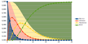
Chances to get veteran ranks for a novice unit after a number of matches survived

Let's consider a simplest case of an action where several units participate: $n$ units in one turn attack one defender. The optimal order of attacking a target is a question out of the scope of this article, presume that the order of the attackers is predefined; sending best killer first seems more advantageous for the attacking part for the probability of taking more target's hp before it can get veteran, but unit cost and other considerations may change it. Let each of them has losing limit to defender's defence $l_i$ and attack strength $s_i$, $i=1,...,n$ by the order of attack. What is the chance of the defender to survive the attacks and have hitpoints $d_{{\text{hp}}n}$ afterwards?

To answer this question, we must also take into account the probability $p_{\text{vet}}(v_{i-1})$ for the defender who survived an $i$-th match to get a veteran rank $v_i$ and thus a strength bonus; the defender strength against each one is $r_{i}=r(v_{i-1})$. This rank is in general not independent from $d_{{\text{hp}}n}$ since units that have got the status earlier tend to preserve more hp. The formulation for the possibility of given defender state will be recurrent, based on calculation for cases if the defender has got the latest status in the latest match or earlier:

Failed to parse (syntax error): {\displaystyle \mathrm P(d_{\text{hp}n}=h_n, d_{\text{v}n}=v_n) = \sum_{h_{n-1}=h_n}^{d_{\text{hp}0}}\Big(\\ \mathrm P(d_{\text{hp}n-1}=h_{n-1}, d_{\text{v}n}=v_n-1)p_\text{vet}(v_n-1)\mathrm P(w=\frac{h_{n-1}-h_n}{a_{\text{fp}i}}|h_{n-1},s_i, r(v_n-1),l_i)+\\ \;+\mathrm P(d_{\text{hp}n-1}=h_{n-1}, d_{\text{v}n}=v_n)(1-p_\text{vet}(v_n))\mathrm P(w=\frac{h_{n-1}-h_n}{a_{\text{fp}i}}|h_{n-1},s_i, r(v_n),l_i)\Big)} ,

where probabilities of winning $w$ rounds for attacker (before not winning the match) is calculated by swapping roles in formulae for $d$ above, with zeroes for non-integer parameter values.

Since neither attacker in the series is expected to inflict more then final amount of damage $b=h_{0}-h_{n}=\sum _{i=1}^{n}w_{i}a_{{\text{fp}}i}$ which is less then the defender's health, the actual value of defender's health is not important for this formula (if only there is no bombardment which can possibly beat out in process the last hp); we actually calculate a part of the damage distribution for $d_{{\text{hp}}0}=\infty$. If we fix veteran status for each match and thus $p_{i},q_{i}$ are known, then the order of the attackers does not have any effect on the final results. During bombardment, no unit can increase its veteran status; so, for a series of bombardments we can apply a formula for the damage $b$ they would cause to a unit of endless health and similar strength

$\mathrm {P} _{n}(b)=\sum _{w_{n}=0}^{\lfloor b/a_{\text{fp}}\rfloor }f_{B\;a_{\text{br}},p}(w_{n})P_{n-1}(b-w_{n}a_{\text{fp}})$

and then sum up in one the values that are greater than or equal to $d_{\text{hp}}-1$ and use this number for $d_{{\text{hp}}n}=1$ and the other values for $d_{{\text{hp}}n}=d_{{\text{hp}}0}-b$.

Then, since NBD has additive nature, in the case when firepowers and relative strengthes of two or more attackers are similar and matches with them are "win-or-lose", we can think that we have a single attacker with the same round-winning probability as any single unit and a losing capacity summed from theirs. Alas, sum of negative binomial distributed variables with different parameters is not a NBD variable; it's a mixture of a NBD over another distribution which is not good-looking. Then, distributions of the damage by units with different firepowers are stretched in different scales and are not summated as individual ones. The lucky part is that expected values and variances of independent random variables (what the untruncated damage functions are) are additive, so we can get the estimated mean and try to suggest how would the value go so far with $\Phi \left({\frac {b-\sum \mu _{i}}{\sqrt {\sum \sigma _{i}^{2}}}}\right)$ (but the actual distribution may be much different from a normal one, so this approximation is unstable).

Specifically, if all matches are unlimited and strengthes for each match are supposed to be known, then we can represent the probability of defeating against all the attackers (with fixed result or in total) as probability to win the rounds we must win to overcome each one $Q=\prod _{i=1}^{n}q_{i}^{l_{i}}$, multiplied with the probability of losing them given amount of hp in all possible combinations:

Failed to parse (syntax error): {\displaystyle P_n(b)=\sum\limits_{\sum_{i=1}^n w_i a_{\text{fp}i}=b} \prod_{i=1}^n f_{NB\;q_i,l_i}(w_i) = \\ \;= Q \sum\limits_{\sum_{i=1}^n w_i a_{\text{fp}i}=b} \prod_{i=1}^n {l_i+w_i-1 \choose l_i-1} p_i^{w_i} =\\ \;=Q \sum\limits_{\sum_{i=1}^n w_i a_{\text{fp}i}=b} \frac{\prod_{v=l_{i\min}}^{(l_{i}+w_i)_\max-1}v^{|\{j|l_j\le v < l_j+w_j\}|}}{\prod_{u=1}^{w_{i\max}}u^{|\{j|u\le w_j\}|}} \prod_{i=1}^n p_i^{w_i}}

(formulae for single value, replace $=$ on $\le$ before $b$'s under the sum signs to get cumulative expressions). The recurrent form, however, seems more easy and universal for computing (keeping only as much arrays of reals of length $b+1$ as there are possible veteran ranks plus one buffer is needed to store probabilities of each possible state on any step).

For example, in a common case when we can expect one veteran status change with probability $p_{{\text{vet}}I}$ which changes combat chances from $p_{I},q_{I}$ to $p_{II},q_{II}$ we have to calculate separately matches before and after the status change for watever turn in the middle it happens, and the defender surviving probability will be

Failed to parse (syntax error): {\displaystyle \displaystyle{P_\bar W=(1-p_{\text{vet}I})^{n-1}\sum_{j=0}^{k-1}{L+k-1\choose j}p^j q^{L+k-1-j}+\sum_{i=1}^{n-1}\Big(\\ \;(1-p_{\text{vet}I})^{i-1}p_{\text{vet}I}\sum_{w=0}^{k-1}{L_i+w-1\choose w-1}p_I^w q_I^{L_i} \sum_{j=0}^{k-1-w}{L-L_i+k-1-w\choose j}p_{II}^j q_{II}^{L-L_i+k-1-w-j}\Big)=\\ \;=(1-p_{\text{vet}I})^{n-1}F_{B\;L+k-1,p_I}(k-1)+\\ \;+p_{\text{vet}I}\sum_{i=1}^{n-1}(1-p_{\text{vet}I})^{i-1}q_I^{L_i}\sum_{w=0}^{k-1}{L_i+w-1\choose w-1}p_I^w F_{B\;L_i+k-1-w,p_{II}}}\text,}

where $L_{i}=\sum _{j=1}^{i}l_{j}$. As you can see from the chart, novice units have around one change expected after surviving 1 to 3 matches, two after 4 to 8, and since then they are more likely Elite than not (about 99% likely just after they have survived their 24th battle). Thus, some least possible combinations we can filter out on early stages of computing (especially ones with higher $b$, since combinations can receive probability growth during iterations only by "shifting" from bigger hp).

Approximation

This page is in development. It may lack necessary details and contain information that is not completely accurate.

Without any more sophisticated ways to approximate sum of NBD variables, an approximation using Poisson instead of NBD may be used to estimate the outcome much faster. Denoting untruncated NBD mean for each attacker $E_{i}={\frac {l_{i}p_{i}}{q_{i}}}$, we can consider that $f_{NB\;l_{i},q_{i}}(w_{i})\approx f_{P\;E_{i}}(w_{i})$. The brilliant property of Poisson distribution is that it is additive: if $X_{i}\sim \mathrm {P} (\lambda _{i})$, then $\sum X_{i}\sim \mathrm {P} (\sum \lambda _{i})$. Thus, we can sum up in one all attackers with same firepower; and, since we rarely have in the game firepowers other than 1 and 2, we can reduce the combination of numerous regular attackers to one or two. Some attackers with binomial or mostly binomial damage law also can be with a reasonable precision approximated by Poisson function with $E_{i}=m_{i}q_{i}$, the limitations of this approximation are discussed above (and units with $m_{i}>\lfloor b/a_{{\text{fp}}i}\rfloor$ can be considered unlimited); other units can't be grouped such way but may get fast normal or other approximation. In a group of "Poissonable" attackers,

Failed to parse (syntax error): {\displaystyle P_n(b)\approx\sum\limits_{ \sum_{f\in\{a_{\text{fp}i}\}}fw_f=b } \prod_{f\in\{a_{\text{fp}i}\}}f_{P\;\sum_{a_{\text{fp}i}=f}E_i}(w_f) =\\ \;= \exp{\left(-\sum_{i=1}^{n}E_i\right)} \sum\limits_{\sum fw_f=b} \prod_{f\in\{a_{\text{fp}i}\}} \frac{(\sum_{a_{\text{fp}i}=f}E_i)^{w_f}}{w_f!}=\\ \;= \exp\left(-\sum_{i=1}^{n}E_i\right) \sum\limits_{\sum fw_f=b}\frac{ \exp \sum_{f\in\{a_{\text{fp}i}\}} w_f \ln \sum_{a_{\text{fp}i}=f}E_i }{ \prod_{u=1}^{w_{f\max}}u^{|\{j|u\le w_f\}|}} \text.}

For some better precision, we can also calculate separately the sum of damage by "oneshotable" attackers for which the Poisson approximation works worst and straight calculation works best; for a group of such variables with similar fp we can easily get the losing rounds probability component $S_{n}(w)=\sum _{\sum _{i=1}^{n}w_{i}=w}\prod p_{i}^{w_{i}}$ from the recursion $S_{n}(w+1)={\frac {1}{w+1}}\left(S_{n}(w)S_{n}(1)+w\sum _{i=1}^{n}p_{i}^{w+1}\right)$.

We can also make a rough but quick estimation of winning chance recursively converting the first attacker to fp and strength of the second (avoiding rounding when possible), adding to the defender's health the points the equivalent one takes at average more then the original and combining the first two defenders into one, and take for each step average veteran bonuses, calculated from sum of corresponding bonuses, multiplied on veteran level possibilities; but the precision of such a procedure is not studied yet and seems to be sometimes surprisingly low.

Prolonged 1v1

This page is in development. It may lack necessary details and contain information that is not completely accurate.

Consider now two units with limited combat rounds standing against each other as long as they both live. As you can see on the charts above, units with comparable strength have rather large chance to survive both the attack. After one or two attacks, the attacker will be run off of ovement points/attack limit; then the defender may counter-attack, or just stay in place and wait his hp regenerate a little (and if he stays in a city with Barracks, his hp will be full next turn). And if the battle dures and dures, even unit which has just attacked is considered unmoved and has some HP regeneration, and UNO wonder gives hp anyway. If both are using optimal strategies against each other, the battle might dure long, or will end in a true stalemate if, when both regenerate full hp, their attack odds show up too big to try.

When we consider operations that involve several consequent actions, we need take in account the desirability of the goal for the player regarding the undesirability of obstacles. For each player there is some value for the fact their own unit survived and a price for another player's unit's head (say, for player X against player Y they are $c_{XX},c_{YX}$); if one of the unts protects a valuable city, the prices can be much different even if the units' stats are similar. Even if they don't change much in time, a unit spending turns in this battle probably consumes city resources and/or could do something more useful in another place; thus, if an action which may take several turns is planned, its price should be amortized ("amortization" is a common word arond AI code though it is poorly commented). Another thing is the initiative: if both parts have better odds attacking then defending, one who pushes the button first and has faster modem (or is AI) wins it. Also, the number of attacks possible in one turn for many units (that have more than 1 mp, "DamageSlows" flag and no "OneAttack" flag) is proportional to their health; and, if it happens that they have less than 1 full mp, they may be subject to the "tired_attack" effect: their strength falls proportionally. And if the things were not yet complicated enough, if some of the units sees once that the stand turns bad for him in either attacking or defending, it can leave the battlefield and run away/go to solve any worthy problem (if it has yet enough speed or the opponent can't/doesn't want to chase).

Last variant aside, we can assume the system of two units' state as integer eight-dimensional vector of hp, mp, fortified state and veteran status for each unit, on $i$th turn it is $S_{i}=(h_{X},a_{X},f_{x},v_{X},h_{Y},a_{Y},f_{Y},v_{Y})_{i}$. In the sequence of such vectors, each step means X attack, Y attack or turn change. Attacks lower the attacker's mp on a constant (or less down to 0), then lower hitpoints for both with distributions discussed above with some probability of expelling, then reduce movement points according to DamageSlows and possibly give the survivor(s) veteran growth; for them to happen, the attacker must have nonzero mp and a desire to attack this time; and if these conditions are met simultaneously for both units, attacker must win the initiative. The turn change happens when the conditions are unmet for both sides, it restores the hp and the mp (to the hp-related maximum). Except for the initial state, we can be sure that a fortifiable unit which ended previous turn with nonzero mp and has not attacked yet this turn is fortified (because why not).

For not taking too much in scope, we can assume that the preferability of attack on each step depends only on the units' actual state; then the sequence with total probability 1 in a finite number of turns either ends in death of one of the units or stabilizes in a true stalemate (in both cases veteran status outcome(s) might be different). So, if X considers attack on step 0 when the system is in the state $S_0$ and has planning horizont $i_{\max }$ (let us express it in steps rather than in turns for a bit of simplicity), X's total expected amortized income from this action is

Failed to parse (syntax error): {\displaystyle c_{aX}(S_0)=P_{WXa}(S_0)c_{YX}(1)-P_{LXa}(S_0)c_{YX}(1)+\\ +\sum_{\{S_{1Xa}|h_X>0<h_y\}}\mathrm{P}(S_1=S_{1Xa}|\text{in }S_0 \text{ X decided to attack})\sum_{i=2}^{i_\max}\sum_{\forall S}\mathrm{P}(S_{i-1}=S|S_1=S_{1Xa})\left(P_{WX}(S)c_{YX}(i)-P_{LX}(S)c_{XX}(i)\right)} ,

where $P_{WX}(S),P_{LX}(S)$ are probabilities for X to win and lose after pre-battle condition $S$ (observing chances and wills of both sides to attack); $P_{WXa,LXa}(S_{0})$ are battle outcome probabilities on step 1 if X considers to attack regarding chances and will of Y to intercept. The expected income from deciding to keep on fortifying in the same situation $c_{fX}(S_{0})$ can be expressed in similar way; Y can't disallow X to fortify but considers attacking or also fortifying. If one of the expected incomes is positive and is not less than the another, the unit will take that tactic; if they both are negative, then the unit will try to leave the battle.

The probabilities of given states on given turns are calculated recursively - they are derived from the previous state starting from presumed both-survived result after step 1 $S_{1Xa}$; but to know the process of each step one must first know will the participants attack or leave the battle after given states. That means, if the values of each unit for each side on each turn is known to both sides, then for any state theoretically reachable from the starting conditions there are 4 equations for 4 unknown variables (expected incomes), and signs of differences in two pairs of them govern all the equations for the conditions this condition is accessible from in observed number of steps, itself inclusive.

Literature

• Norman L. Johnson, Adrienne W. Kemp, Samuel Kotz.

Univariate Discrete Distributions. 2005

• Shonkwiler, J.S., Variance of the truncated negative binomial

distribution. Journal of Econometrics (2016)

• Ken Butler, Michael Stephens. The distribution of a sum of binomial random variables. 1993
• Furman E. On the convolution of the negative binomial random variables. 2006